

勉強がてら日経平均を使って簡易のバックテストをしてみるのでまとめておきます。
はじめに
まず参考書籍を紹介しておきます。何冊か本を読みましたがこのオライリーのPythonによるファイナンス第二版が特に読みやすかったです。

Pythonによるファイナンス 第2版 ―データ駆動型アプローチに向けて (オライリー・ジャパン)
バックテストに関する本は何冊か読みましたが難しめのものが多く初心者だと挫折しがちですがこの本ではPythonの基本的な文法から始まってpandas,numpyから機械学習、ディープラーニングまで広く扱っておりバックテストや自動取引を始める場合一番良書だと思いますので自信をもっておすすめできます。
またPythonでFXシストレバックテストのサイトも参考にしました。
1.データの入手
前回同様データの入手はYAHOOファイナンスからで、取得方法は過去の記事を参照してください。
2.前処理
2.1 読み込み
データをread_csvで読み込みます。sep=’,’でカンマで区切っているデータを指定します。namesで列名を指定。使用するデータはCloseまでですのでusecolsで範囲を指定することで左から5列目までのデータを使用することを指定します。index_colはインデックス列を指定して、parse_datesでdatetime型に変更します。最後にheader=0でヘッダー行も指定しています。
import numpy as np
import pandas as pd

df = pd.read_csv('^N225m.csv',
                     sep=',',
                     names=('Date','Open','High','Low','Close'),
                     usecols=range(5),
                     index_col=0,
                     parse_dates=True,
                     header=0)
print(df.head())
結果・・・データフレームにcsvが正しく読み込まれたことがわかります。
                   Open         High          Low        Close
Date
1965-01-05  1257.719971  1257.719971  1257.719971  1257.719971
1965-01-06  1263.989990  1263.989990  1263.989990  1263.989990
1965-01-07  1274.270020  1274.270020  1274.270020  1274.270020
1965-01-08  1286.430054  1286.430054  1286.430054  1286.430054
1965-01-12  1288.540039  1288.540039  1288.540039  1288.540039
2.2 時間軸変更
取得したデータは日足ですがここでは週足に変更します。pandasのresample()メソッドを使います。label引数は開始日にするか終了日にするかを決めます。closed引数は開始日と終了日のどちらの期間を含むかを指定します。
ohlc = {'Open': 'first',
          'High': 'max',
          'Low': 'min',
          'Close': 'last'}

df_W=df.resample('W', closed='left', label='left').agg(ohlc)
print(df_W)
結果。これで週足に変更することができました。
                    Open          High           Low         Close
Date
1965-01-03   1257.719971   1286.430054   1257.719971   1286.430054
1965-01-10   1288.540039   1289.500000   1281.670044   1289.500000
1965-01-17   1271.680054   1271.680054   1261.829956   1261.829956
1965-01-24   1249.719971   1258.209961   1242.270020   1242.270020
1965-01-31   1242.829956   1263.589966   1238.750000   1263.589966
...                  ...           ...           ...           ...
2019-07-07  21665.789063  21720.140625  21488.220703  21685.900391
2019-07-14  21644.380859  21655.519531  20993.439453  21466.990234
2019-07-21  21394.750000  21823.070313  21317.849609  21658.150391
2019-07-28  21627.550781  21792.980469  20960.089844  21087.160156
2019-08-04  20909.980469  20941.830078  20110.759766  20684.820313

[2849 rows x 4 columns]
2.3インジケータ作成
続いてインジケータを作成します。ここでは簡単に移動平均線の関数を定義します。pandasのrollingメソッドを使えば簡単に作れます。元データdataと期間periodを引数にした関数で次のように定義できます。
def SMA(data,period):
    sma = data['Close'].rolling(period).mean()
    return sma
SMA_5=SMA(df_W,5)
print(SMA_5)
Date
1965-01-03 NaN
1965-01-10 NaN
1965-01-17 NaN
1965-01-24 NaN
1965-01-31 1268.723999
...
2019-07-07 21416.746484
2019-07-14 21486.766406
2019-07-21 21566.668359
2019-07-28 21528.916406
2019-08-04 21316.604297
Freq: W-SUN, Name: Close, Length: 2849, dtype: float644週目まではNaNで5週目に平均値が計算されています。
3週移動平均線も追加してデータフレームdf_Wに追加しておきます。
SMA_3=SMA(df_W,3)
df_W['SMA_5']=SMA_5
df_W['SMA_3']=SMA_3
print(df_W.head())
Open High Low Close SMA_5 \
Date
1965-01-03 1257.719971 1286.430054 1257.719971 1286.430054 NaN
1965-01-10 1288.540039 1289.500000 1281.670044 1289.500000 NaN
1965-01-17 1271.680054 1271.680054 1261.829956 1261.829956 NaN
1965-01-24 1249.719971 1258.209961 1242.270020 1242.270020 NaN
1965-01-31 1242.829956 1263.589966 1238.750000 1263.589966 1268.723999
SMA_3
Date
1965-01-03 NaN
1965-01-10 NaN
1965-01-17 1279.253337
1965-01-24 1264.533325
1965-01-31 1255.896647 3.移動平均線グラフ表示
次に移動平均線と終値をグラフで表示します。ここでは直近100週分の終値とそれぞれ追加した平均線を表示させます。グラフ表示はpandasのplotメソッドを使います。
df_W.iloc[-100:,3:6].plot()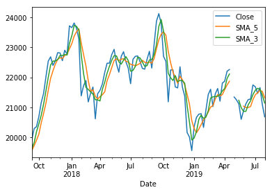
直近100週でなく特定の期間を
例えば2010年2月と3月を表示させてみます。行列の番号ではなく名称で抽出するにはlocメソッドを使います。
df_W.loc['2010-2':'2010-3','Close':'SMA_3'] .plot() 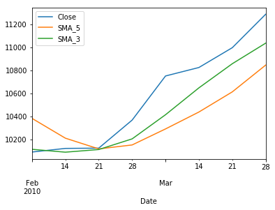
4.バックテスト
バックテストの関数は参考サイトのコードを参照します。売買のルールは3週移動平均線と5週移動平均線ののゴールデンクロスで買い、デッドクロスで売りとします。取引の単位は1として取引手数料はかからないものとします。
FastMA=SMA(df_W,3)
SlowMA=SMA(df_W,5)

#買いエントリーシグナル
BuyEntry = ((FastMA > SlowMA) & (FastMA.shift() <= SlowMA.shift())).values
#売りエントリーシグナル
SellEntry = ((FastMA < SlowMA) & (FastMA.shift() >= SlowMA.shift())).values
#買いエグジットシグナル
BuyExit = SellEntry.copy()
#売りエグジットシグナル
SellExit = BuyEntry.copy()

def Backtest(data, BuyEntry, SellEntry, BuyExit, SellExit,  lots=1):
    Open = data['Open'].values
    Point = 1.0
    Lots=lots*1.0
    N = len(data)
    BuyEntry[N-2] = SellEntry[N-2] = True
    BuyPrice = SellPrice = 0.0

    LongTrade = np.zeros(N)
    ShortTrade = np.zeros(N)

    LongPL = np.zeros(N)
    ShortPL = np.zeros(N)

    for i in range(1,N):
        if BuyEntry[i-1] and BuyPrice ==0:
            BuyPrice = Open[i]
            LongTrade[i] = BuyPrice
        elif BuyExit[i-1] and BuyPrice !=0:
            ClosePrice = Open[i]
            LongTrade[i] = -ClosePrice
            LongPL[i] = (ClosePrice - BuyPrice)*Lots
            BuyPrice = 0

        if SellEntry[i-1] and SellPrice == 0:
            SellPrice = Open[i]
            ShortTrade[i] = SellPrice
        elif SellExit[i-1] and SellPrice !=0:
            ClosePrice = Open[i]
            ShortTrade[i] = -ClosePrice
            ShortPL[i] = (SellPrice - ClosePrice)*Lots
            SellPrice = 0

    return pd.DataFrame({'Long':LongTrade, 'Short':ShortTrade}, index = data.index),\
            pd.DataFrame({'Long':LongPL, 'Short':ShortPL}, index = data.index)

Trade, PL = Backtest(df_W, BuyEntry, SellEntry, BuyExit, SellExit)
5.損益評価
バックテストの結果を評価します。こちらも参考サイトのコードをに若干修正を加えたものを使用します。
def BacktestReport(Trade, PL):
    LongPL = PL['Long']
    LongTrades = np.count_nonzero(Trade['Long'])//2
    LongWinTrades = np.count_nonzero(LongPL.clip(lower=0))
    LongLoseTrades = np.count_nonzero(LongPL.clip(upper=0))
    print('買いトレード数 =', LongTrades)
    print('勝トレード数 =', LongWinTrades)
    print('最大勝トレード =', LongPL.max())
    print('平均勝トレード =', round(LongPL.clip(lower=0).sum()/LongWinTrades, 2))
    print('負トレード数 =', LongLoseTrades)
    print('最大負トレード =', LongPL.min())
    print('平均負トレード =', round(LongPL.clip(upper=0).sum()/LongLoseTrades, 2))
    print('勝率 =', round(LongWinTrades/LongTrades*100, 2), '%\n')

    ShortPL = PL['Short']
    ShortTrades = np.count_nonzero(Trade['Short'])//2
    ShortWinTrades = np.count_nonzero(ShortPL.clip(lower=0))
    ShortLoseTrades = np.count_nonzero(ShortPL.clip(upper=0))
    print('売りトレード数 =', ShortTrades)
    print('勝トレード数 =', ShortWinTrades)
    print('最大勝トレード =', ShortPL.max())
    print('平均勝トレード =', round(ShortPL.clip(lower=0).sum()/ShortWinTrades, 2))
    print('負トレード数 =', ShortLoseTrades)
    print('最大負トレード =', ShortPL.min())
    print('平均負トレード =', round(ShortPL.clip(upper=0).sum()/ShortLoseTrades, 2))
    print('勝率 =', round(ShortWinTrades/ShortTrades*100, 2), '%\n')

    Trades = LongTrades + ShortTrades
    WinTrades = LongWinTrades+ShortWinTrades
    LoseTrades = LongLoseTrades+ShortLoseTrades
    print('総トレード数 =', Trades)
    print('勝トレード数 =', WinTrades)
    print('最大勝トレード =', max(LongPL.max(), ShortPL.max()))
    print('平均勝トレード =', round((LongPL.clip(lower=0).sum()+ShortPL.clip(lower=0).sum())/WinTrades, 2))
    print('負トレード数 =', LoseTrades)
    print('最大負トレード =', min(LongPL.min(), ShortPL.min()))
    print('平均負トレード =', round((LongPL.clip(upper=0).sum()+ShortPL.clip(upper=0).sum())/LoseTrades, 2))
    print('勝率 =', round(WinTrades/Trades*100, 2), '%\n')

    GrossProfit = LongPL.clip(lower=0).sum()+ShortPL.clip(lower=0).sum()
    GrossLoss = LongPL.clip(upper=0).sum()+ShortPL.clip(upper=0).sum()
    Profit = GrossProfit+GrossLoss
    Equity = (LongPL+ShortPL).cumsum()
    MDD = (Equity.cummax()-Equity).max()
    print('総利益 =', round(GrossProfit, 2))
    print('総損失 =', round(GrossLoss, 2))
    print('総損益 =', round(Profit, 2))
    print('プロフィットファクター =', round(-GrossProfit/GrossLoss, 2))
    print('平均損益 =', round(Profit/Trades, 2))
    print('最大ドローダウン =', round(MDD, 2))
    print('リカバリーファクター =', round(Profit/MDD, 2))
    return Equity
Equity = BacktestReport(Trade, PL)
買いトレード数 = 285
勝トレード数 = 138
最大勝トレード = 6662.708984000001
平均勝トレード = 667.3
負トレード数 = 147
最大負トレード = -4082.0898439999983
平均負トレード = -427.56
勝率 = 48.42 %
売りトレード数 = 284
勝トレード数 = 114
最大勝トレード = 6356.980468000002
平均勝トレード = 661.13
負トレード数 = 170
最大負トレード = -2032.6191409999992
平均負トレード = -387.17
勝率 = 40.14 %
総トレード数 = 569
勝トレード数 = 252
最大勝トレード = 6662.708984000001
平均勝トレード = 664.51
負トレード数 = 317
最大負トレード = -4082.0898439999983
平均負トレード = -405.9
勝率 = 44.29 %
総利益 = 167455.74
総損失 = -128669.34
総損益 = 38786.41
プロフィットファクター = 1.3
平均損益 = 68.17
最大ドローダウン = 7402.96
リカバリーファクター = 5.24この結果だけ見ると総損益38786円、プロフィットファクター1.3なので単純なロジックでもそこまで悪くない結果といえそうです。
7.損益のグラフ化
matplotlibのライブラリを読み込んでグラフ化しておきます。
import matplotlib as mpl
import matplotlib.pyplot as plt

plt.plot(Equity)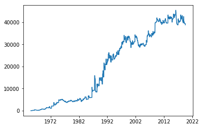
8.指値注文でバックテスト
バックテストにもう少し機能を拡張します。TP(Take Profit:利食い)とSL(Stop Loss:損切)、Limit(指値)をそれぞれ追加します。単位は%です。指値0.5%,利食い8%損切20%でまずテストします。
def Backtest_rev(ohlc, BuyEntry, SellEntry, BuyExit, SellExit, lots=100,  TP=10, SL=10, Limit=5, Expiration=10):
    Open = ohlc.Open.values #始値
    Low = ohlc.Low.values #安値}
    High = ohlc.High.values #高値
    Lots = lots #実際の売買量
    N = len(ohlc) #データのサイズ

    LongTrade = np.zeros(N) #買いトレード情報
    ShortTrade = np.zeros(N) #売りトレード情報

    BuyEntryS=np.hstack((False,BuyEntry[:-1]))
    if Limit ==0: LongTrade[BuyEntry]=Open[BuyEntryS]
    else: #指値買い
        for i in range(N-Expiration):
            if BuyEntryS[i]:
                BuyLimit = Open[i]-Limit/100*Open[i] #指値
                for j in range(Expiration):
                    if Low[i+j] <= BuyLimit: #約定条件
                        LongTrade[i+j] = BuyLimit
                        break
    #買いエグジット価格
    BuyExitS = np.hstack((False, BuyExit[:-2], True)) #買いエグジットシグナルのシフト
    LongTrade[BuyExitS] = -Open[BuyExitS]

    #売りエントリー価格
    SellEntryS = np.hstack((False, SellEntry[:-1])) #売りエントリーシグナルのシフト
    if Limit == 0: ShortTrade[SellEntryS] = Open[SellEntryS] #成行売り
    else: #指値売り
        for i in range(N-Expiration):
            if SellEntryS[i]:
                SellLimit = Open[i]+Limit/100*Open[i] #指値
                for j in range(Expiration):
                    if High[i+j] >= SellLimit: #約定条件
                        ShortTrade[i+j] = SellLimit
                        break
    #売りエグジット価格
    SellExitS = np.hstack((False, SellExit[:-2], True)) #売りエグジットシグナルのシフト
    ShortTrade[SellExitS] = -(Open[SellExitS])

    LongPL = np.zeros(N) # 買いポジションの損益
    ShortPL = np.zeros(N) # 売りポジションの損益
    BuyPrice = SellPrice = 0.0 # 売買価格

    for i in range(1,N):
        if LongTrade[i] > 0: #買いエントリーシグナル
            if BuyPrice == 0:
                BuyPrice = LongTrade[i]
                ShortTrade[i] = -BuyPrice #売りエグジット
            else: LongTrade[i] = 0

        if ShortTrade[i] > 0: #売りエントリーシグナル
            if SellPrice == 0:
                SellPrice = ShortTrade[i]
                LongTrade[i] = -SellPrice #買いエグジット
            else: ShortTrade[i] = 0

        if LongTrade[i] < 0: #買いエグジットシグナル
            if BuyPrice != 0:
                LongPL[i] = -(BuyPrice+LongTrade[i])*Lots #損益確定
                BuyPrice = 0
            else: LongTrade[i] = 0

        if ShortTrade[i] < 0: #売りエグジットシグナル
            if SellPrice != 0:
                ShortPL[i] = (SellPrice+ShortTrade[i])*Lots #損益確定
                SellPrice = 0
            else: ShortTrade[i] = 0

        if BuyPrice != 0 and SL > 0: #SLによる買いポジションの決済
            StopPrice = BuyPrice-SL/100*BuyPrice
            if Low[i] <= StopPrice:
                LongTrade[i] = -StopPrice
                LongPL[i] = -(BuyPrice+LongTrade[i])*Lots #損益確定
                BuyPrice = 0

        if BuyPrice != 0 and TP > 0: #TPによる買いポジションの決済
            LimitPrice = BuyPrice+TP/100*BuyPrice
            if High[i] >= LimitPrice:
                LongTrade[i] = -LimitPrice
                LongPL[i] = -(BuyPrice+LongTrade[i])*Lots #損益確定
                BuyPrice = 0

        if SellPrice != 0 and SL > 0: #SLによる売りポジションの決済
            StopPrice = SellPrice+SL/100*SellPrice
            if High[i] >= StopPrice:
                ShortTrade[i] = -StopPrice
                ShortPL[i] = (SellPrice+ShortTrade[i])*Lots #損益確定
                SellPrice = 0

        if SellPrice != 0 and TP > 0: #TPによる売りポジションの決済
            LimitPrice = SellPrice-TP/100*SellPrice
            if Low[i] <= LimitPrice:
                ShortTrade[i] = -LimitPrice
                ShortPL[i] = (SellPrice+ShortTrade[i])*Lots #損益確定
                SellPrice = 0

    return pd.DataFrame({'Long':LongTrade, 'Short':ShortTrade}, index=ohlc.index),\
            pd.DataFrame({'Long':LongPL, 'Short':ShortPL}, index=ohlc.index)

Trade, PL = Backtest_rev(df_W, BuyEntry, SellEntry, BuyExit, SellExit, TP=8, SL=20, Limit=0.5)
Equity2 = BacktestReport(Trade, PL)
plt.plot(Equity2)
買いトレード数 = 221
勝トレード数 = 99
最大勝トレード = 282539.79578324
平均勝トレード = 48194.69
負トレード数 = 122
最大負トレード = -383965.37893099996
平均負トレード = -39865.53
勝率 = 44.8 %
売りトレード数 = 227
勝トレード数 = 92
最大勝トレード = 248005.78148136009
平均勝トレード = 56517.17
負トレード数 = 136
最大負トレード = -232779.63870950008
平均負トレード = -36022.89
勝率 = 40.53 %
総トレード数 = 448
勝トレード数 = 191
最大勝トレード = 282539.79578324
平均勝トレード = 52203.42
負トレード数 = 258
最大負トレード = -383965.37893099996
平均負トレード = -37839.95
勝率 = 42.63 %
総利益 = 9970853.71
総損失 = -9762707.44
総損益 = 208146.27
プロフィットファクター = 1.02
平均損益 = 464.61
最大ドローダウン = 957376.95
リカバリーファクター = 0.22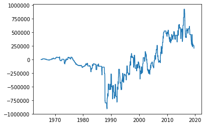
最終的にはプラスになっていますが途中でバブル期のドローダウンが耐えられる気がしません。
続いてTP=20%,SL=1%とした場合
買いトレード数 = 164
勝トレード数 = 48
最大勝トレード = 394416.67968799995
平均勝トレード = 64153.94
負トレード数 = 179
最大負トレード = -37132.933593750204
平均負トレード = -12717.07
勝率 = 29.27 %

売りトレード数 = 165
勝トレード数 = 46
最大勝トレード = 427862.65430189995
平均勝トレード = 63699.89
負トレード数 = 185
最大負トレード = -37037.374921875016
平均負トレード = -12589.51
勝率 = 27.88 %

総トレード数 = 329
勝トレード数 = 94
最大勝トレード = 427862.65430189995
平均勝トレード = 63931.74
負トレード数 = 364
最大負トレード = -37132.933593750204
平均負トレード = -12652.24
勝率 = 28.57 %

総利益 = 6009583.88
総損失 = -4605415.03
総損益 = 1404168.85
プロフィットファクター = 1.3
平均損益 = 4267.99
最大ドローダウン = 359975.06
リカバリーファクター = 3.9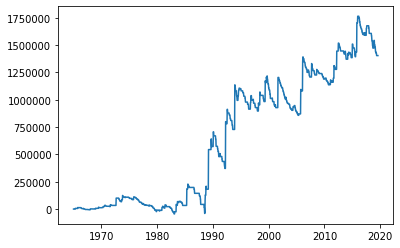
バブルのころのドローダウンもほとんどなくPFも1.3と大きく向上しました。いろいろとパラメータを変えてみると面白い結果が得られそうです。
9.まとめ
今回は単純なゴールデンクロス・デッドクロスで日経平均をバックテストしてみました。1965年からと期間が長すぎるのと初期の資金、買い付け余力や手数料等の条件が何もないのでこの結果の評価の仕方について検討の余地があると思います。この二つの結果だけみれば一般的に言われている損小利大のトレードをしたほうが優位性があるということ言えそうです。
この記事は一旦ここまでとします。


コメント